Working with discrete data

Even though ennemi was originally designed to handle continuous variables, it can estimate MI between discrete variables as well. Very usefully, it can also estimate the dependence between discrete and continuous variables.

In this tutorial, we will apply ennemi to a very simplified example. You can download the source code for this example to play with the model.

A very simple weather model

In the fictional town of Entropyville, the weather is very straightforward: either it rains, is partly cloudy, or is perfectly clear.

Example plot: higher temperatures correlate with sunny weather

The weather is fairly stable, and as such it is enough to look at weekly values. We have 200 weeks of weather data at our disposal, stored in a pandas data frame:

print(data)

    Weather  Temp   Press Wind
   rainy   9.0  1002.0    W
   rainy  16.0  1008.0    N
   clear  17.0  1028.0    E
  cloudy  17.0  1027.0    S
   clear  21.0  1030.0    W
..      ...   ...     ...  ...
cloudy  11.0  1031.0    S
cloudy  14.0  1021.0    N
cloudy  14.0  1002.0    N
 rainy  10.0   998.0    W
 rainy  19.0   990.0    W

Let’s start finding out how to forecast the next week!

Note for `pandas` users

String data in a pandas data frame must be fixed up. This step is not necessary with raw NumPy arrays.

The problem is that pandas stores strings internally as the object data type. This data type cannot be used in the estimation of MI. We can convert the categories to integers to fix the problem.

# Not the most optimal code, but sufficient in small example
data2 = data.drop(columns=["Weather", "Wind"])

data2["Wind"] = 0
data2.loc[data["Wind"] == "E", "Wind"] = 1
data2.loc[data["Wind"] == "S", "Wind"] = 2
data2.loc[data["Wind"] == "W", "Wind"] = 3

data2["Weather"] = 0
data2.loc[data["Weather"] == "cloudy", "Weather"] = 1
data2.loc[data["Weather"] == "clear", "Weather"] = 2

print(data2)
print(data2.dtypes)

This outputs

     Temp   Press  Wind  Weather
0     9.0  1002.0     3        0
1    16.0  1008.0     0        0
2    17.0  1028.0     1        2
3    17.0  1027.0     2        1
4    21.0  1030.0     3        2
..    ...     ...   ...      ...
195  11.0  1031.0     2        1
196  14.0  1021.0     0        1
197  14.0  1002.0     0        1
198  10.0   998.0     3        0
199  19.0   990.0     3        0

[200 rows x 4 columns]
Temp      float64
Press      float64
Wind         int64
Weather      int64
dtype: object

Correlation between measurements and weather

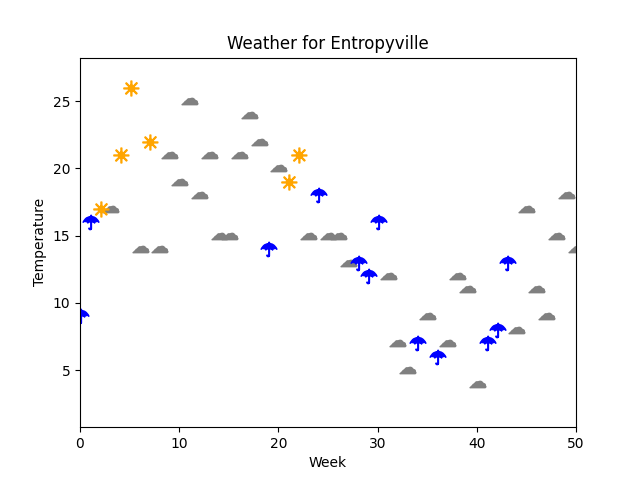
From the figure, it appears likely that temperature has a big role in the weather. Here the two variables are mixed:

Temperature is continuous: it ranges roughly between 0 and 30 degrees (C). Even though the measured values are rounded to whole numbers, we can think of its values as an unbroken scale.
Weather is discrete: it is divided into three categories. We have to assume that there are no in-between values; the data does not give more details.

ennemi can estimate the MI of a discrete-continuous pair just fine, but we have to be careful in its interpretation. The first part is no harder than:

print(estimate_mi(data2["Weather"], data2[["Temp", "Press"]], discrete_y=True))

Note that we passed the discrete_y parameter to indicate that Weather is a discrete variable. (Perhaps confusingly, ennemi calls the first parameter y and the second x. This is because y is the variable of interest, and multiple covariates may be passed in x.)

The code prints

       Temp    Press
0  0.092366  0.07407

But what do these numbers mean? We did not pass normalize=True, so it is not a correlation coefficient. Neither would that parameter help, because it would assume both variables to be continuous.

We have to go back to the theoretical background of MI. MI is measured in nats, an unit of information. It tells us how much information we have about Weather given that we know Temp or Press. So the question should be: how much information there is to know?

We can estimate the information content, also known as entropy, of Weather by calling

print(estimate_entropy(data2["Weather"], discrete=True))

    Weather
0  0.905266

That is, out of the 0.91 nats of information, temperature provides only 0.092 nats, and air pressure even less.

Note: The entropy of a continuous variable is interpreted very differently. In particular, one cannot compare ratios of entropies like we do below.

Conditioning on the other variable

We can use conditioning to answer the question:

If I already know the temperature, how much extra information on weather does air pressure give?

This is done by passing the temperature as a conditioning variable:

print(estimate_mi(data2["Weather"], data2["Press"], cond=data2["Temp"], discrete_y=True))

The amount of information has increased:

      Press
0  0.144797

What does this mean, then? Recall that the temperature alone gave 0.092 nats of information. Knowing also the air pressure gives 0.145 nats more – meaning that the total knowledge is already 0.237 nats. Together, the two variables explain 26 % of the weather.

In the literature, this is also known as the uncertainty coefficient.

Correlation between wind direction and weather

Let us consider another pair of variables for a moment: the wind direction might have something to do with the weather too.

print(estimate_mi(data2["Weather"], data2["Wind"], discrete_y=True, discrete_x=True))

Now we passed the discrete_x parameter to mark the Wind variable as discrete too. (For the time being, estimate_mi does not allow mixing continuous and discrete x covariates.)

The results are very promising:

       Wind
0  0.533151

Wind direction alone seems to explain most (59 %) of the randomness in weather. Moreover, wind at Entropyville seems to be independent of the other measures:

print(estimate_mi(data2["Wind"], data2[["Temp", "Press"]], discrete_y=True))

       Temp     Press
0  0.026497 -0.008977

The values are practically zero. (Even though MI is always non-negative, ennemi passes the estimation error through. This explains the negative value for the air pressure.)

Limitations in conditioning

It would be tempting to repeat the previous exercise of conditioning. However, this code gives a warning:

print(estimate_mi(data2["Weather"], data2["Wind"],
      cond=data2[["Temp","Press"]], discrete_y=True, discrete_x=True))

UserWarning: A discrete variable has relatively many unique values. Have you set marked the discrete variables in correct order? If both X and Y are discrete, the conditioning variable cannot be 
continuous (this limitation can be lifted in the future).

As of version 1.3, ennemi supports only these combinations of variables and conditions:

	No condition	Discrete	Continuous	Both types in 2D condition
Discrete-discrete	✔️	✔️	❌	❌
Discrete-continuous	✔️	❌	✔️	❌
Continuous-continuous	✔️	❌	✔️	❌

Future versions of ennemi may implement the estimation for more combinations.

Luckily for our example, we already got a lot of information:

Wind direction gives 0.53 nats;
Air pressure and temperature together give 0.24 nats;
There is little to no overlap between these two.

That is, we have explained 85 % of the variation in weather. The remaining 0.14 nats give fairly little random variation: they correspond roughly to getting 1 on a 30-sided die.

Pairwise correlations

For completeness, let us redo the individual estimates in a more efficient manner. The pairwise_mi method is designed to give an efficient overview of the variable relations.

print(pairwise_mi(data2, discrete=[False, False, True, True]))

Here the discrete parameter corresponds to the columns of the data frame. The output is a matrix of pairwise MIs:

             Temp     Press      Wind   Weather
Temp          NaN -0.031239  0.026497  0.092366
Press   -0.031239       NaN -0.008977  0.074070
Wind     0.026497 -0.008977       NaN  0.533151
Weather  0.092366  0.074070  0.533151       NaN

In particular, the last column (or row) gives the values that we calculated earlier. We also see that the other variables are independent of each other.

On interpretation: The matrix entries corresponding to continuous-continuous variable pairs should be interpreted differently to the others. In particular, they should be converted to a correlation coefficient. As correlation coefficients and MI values cannot be directly compared, ennemi does not do this automatically.

Conditioning: Due to the limitations mentioned above, pairwise_mi does not support conditioning when the data contains both discrete and continuous variables.

Conclusion

Even though this was a silly toy example with generated data (and a very unrealistic model of weather!), we went through the relevant estimation methods. We also discussed one way of interpreting the data.

In this tutorial, we did not look into autocorrelation, time lags, or masking. These features work just as in the general tutorial.