What is entropy?

There are many textbooks and articles on entropy and mutual information, not to forget Wikipedia. Because of that, this page does not go into the details. Instead, we only build enough intuition to understand the internals of ennemi.

A discrete example

You are probably familiar with bits, the 0s and 1s computers speak in. There are several derivative units, like byte, equal to 8 bits. With one byte, you can express $2^8 = 256$ different values.

The entropy of a discrete random variable is simply the average number of bits needed to express its value. If the random variable has 256 equally likely values, its entropy is 8 bits. But if the random variable is \(\begin{cases} 0, &\text{with probability } \frac 1 2,\\ 1, \ldots, 255, &\text{with probability} \frac{1}{510}, \end{cases}\) the entropy is about 5 bits. This is because in half of the cases, the variable can be expressed with just one bit: $0$. In the rest of the cases, we can use nine bits: a $1$ for distinction from the first case, followed by eight bits that encode the value. On average, we thus need $1 \cdot \frac 1 2 + 9 \cdot \frac 1 2 = 5$ bits. (This is a simplification; the real entropy computed below is slightly smaller.)

This is how data compression works. A file can be compressed down to as many bits as it has entropy. Each byte in a text file may represent any one of 256 values, but only a fraction of those is used in English text. Moreover, only some combinations of characters are used in English, further reducing the entropy.

Mathematically, the entropy of a random variable $X$ is defined as \(H(X) = \mathbb E \log p(x) = \sum_{x} p(x) \log p(x).\)

The unit of entropy depends on the base we choose for the logarithm. We get bits by using $\log_2$, but generally the natural (base-$e$) logarithm is used. This unit is called nats, and it is used by ennemi.

To convert between bits and nats, we can apply the change-of-base formula: \(\text{bits} = \frac{\text{nats}}{\log_e 2}.\)

To estimate the entropy of a discrete data set, you can call ennemi’s estimate_entropy() method with the parameter discrete=True. The two examples above are computed as in:

from ennemi import estimate_entropy
import numpy as np

data1 = np.arange(0, 256)
entropy1 = estimate_entropy(data1, discrete=True)

print(f"Entropy of first data set: {entropy1:.2f} nats")
print(f"Entropy of first data set: {entropy1 / np.log(2):.2f} bits")

data2 = np.concatenate((np.repeat(0, 256), np.arange(1, 256)))
entropy2 = estimate_entropy(data2, discrete=True)

print(f"Entropy of second data set: {entropy2:.2f} nats")
print(f"Entropy of second data set: {entropy2 / np.log(2):.2f} bits")

Going continuous

If $X$ is a continuous random variable, the natural way to define its entropy is \(H(X) = \mathbb E \log p(x) = \int_\Omega p(x) \log p(x) \,dx.\) However, this definition leads to one significant difference.

As an example, it is easy to calculate that the uniform distribution on the interval ${[{a}, {b}]}$ has entropy equal to $\log (b-a)$. This means that \(H(\mathrm{Uniform(0, 1)}) = 0,\) and even more confusingly \(H(\mathrm{Uniform(0, 1/2)}) = -1 \text{ bits} \approx -0.69 \text{ nats}.\)

Continuous random variables always take on infinitely many values. Therefore we always need an infinite number of bits to express the value.

Instead of being an absolute measure of information like in the discrete case, continuous (or differential) entropy is a relative measure. It tells that you need one coin flip less to express $\mathrm{Uniform(0, 1/2)}$ than $\mathrm{Uniform(0, 1)}$, but both are “at an infinite offset” to zero entropy.

ennemi can estimate the entropy of continuous random variables via the estimate_entropy() method. The variables can be one- or $n$-dimensional.

uniform = np.random.default_rng(0).uniform(0, 0.5, 2000)
print(f"Entropy for Uniform(0, 0.5) variable is {estimate_entropy(uniform):.5f} nats")

Mutual information

Mutual information (MI) answers the question,

If I know the value of $X$, how much is my uncertainty on $Y$ reduced?

MI is defined as \(\mathrm{MI}(X; Y) = H(X) + H(Y) - H(X, Y).\) Intuitively, if you drew a Venn diagram of the two random variables, the mutual information would give the size of their intersection. MI is a relative measure.

MI is useful because it describes the strength of relation between two variables, regardless of the type of relation. For example, consider the below scatter plot:

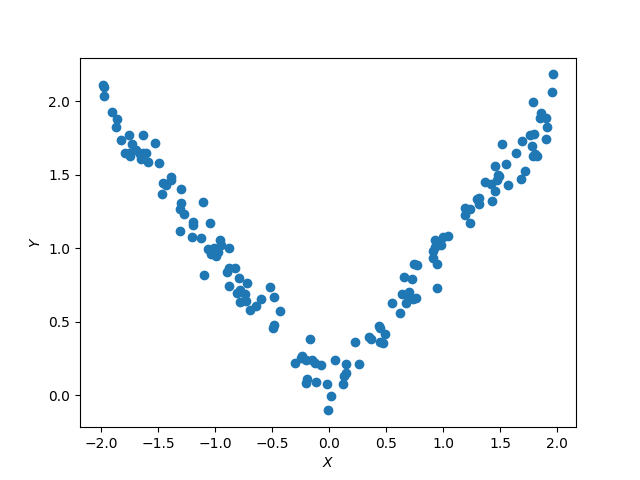
It is pretty obvious that the $X$ and $Y$ variables are related. Specifically, $Y$ seems to be the absolute value of $X$ added with some noise. Yet the classical Pearson correlation coefficient between the two is close to 0. This is because it is calculated by drawing a straight line through the data points.

If, and only if, the variables $X$ and $Y$ are independent, their mutual information is zero. This makes MI a test for independence.

MI is not affected by monotonic transformations of the variables $X$ and $Y$. Additionally, MI is always non-negative (save for estimation errors) and $\mathrm{MI}(X; Y) = \mathrm{MI}(Y; X)$.

Because MI does not depend on the type of correlation, it is very suitable for exploring the dependencies between variables. The ennemi package is designed for this workflow:

1. Calculate the MI between $Y$ and many candidate variables. With time series data, various time lags may be tried. The methods to use are pairwise_mi() and estimate_mi().
2. Select the variables with highest MI for further evaluation.
3. Using MI and conditional MI, further narrow the set of variables.
4. Analyze the dependencies with scatter plots and theoretical knowledge.

The conditional MI mentioned in Step 3 slightly extends the definition:

Given a variable $Z$, how much extra information on $Y$ I gain from $X$?

To quote the classic example, there is a positive correlation between ice cream sales and forest fires. This means that $\mathrm{MI}(\text{fires}; \text{ice cream sales}) > 0$. Of course, both variables depend on the temperature, so we also have $\mathrm{MI}(\text{fires}; \text{temperature}) > 0$ and $\mathrm{MI}(\text{ice cream sales}; \text{temperature}) > 0$.

To find out whether there is any link between forest fires and ice cream, we calculate the MI conditioned on temperature. This removes the effect explained by temperature alone. If \(\mathrm{MI}(\text{forest fires}; \text{ice cream sales} \mid \text{temperature}) > 0,\) there is an actual link. If the conditional MI is zero, the correlation is fully explained by temperature.

Correlation coefficient

Because MI has values in the interval ${[{0},{\infty})}$, it might be hard to interpret. Luckily, there is a way to convert the values to the scale ${[{0},{1})}$ just like with classical correlation methods.

The MI between two normally distributed variables $(X, Y)$ with correlation coefficient $\rho$ is \(\mathrm{MI}(X;Y) = -\frac 1 2 \log (1 - \rho^2).\) This can be solved to give \(\rho = \sqrt{1 - \exp(-2\, \mathrm{MI}(X;Y))}.\)

Do note that this coefficient is exactly equal to the Pearson correlation coefficient in a linear model. However, this gets even better. Remember that MI does not change when the variables are transformed monotonically. This coefficient is equal to the Pearson correlation of the linearized model.

For example, let’s assume that $Y = |X| + \varepsilon$ as in the plot above. The Pearson correlation between $X$ and $Y$ is really low, whereas the correlation between $|X|$ and $Y$ is really high. The MI correlation coefficient is equal to the latter in both cases, correctly suggesting that there is a strong dependency.

The same normalization formula works with conditional MI too, and is equivalent to the partial correlation coefficient. ennemi.estimate_corr() outputs correlation scale values.

The ways of estimation

The most accurate way of estimating entropy or mutual information is to use the definition. This gives the exact value. Unfortunately, for this you need to know the distributions of the variables, which rarely is the case with real-world data. Additionally, closed-form expressions for MI are available only for some well-behaved distributions, such as the multivariate normal distribution: \(\mathrm{MI}(\mathrm{Normal}(\mu, \Sigma)) = -\frac 1 2 \log(\det\Sigma).\)

A common method is to approximate the distribution as a sum of normal distributions. This is called kernel density estimation. However, the accuracy is very sensitive to the bandwidth parameter. Finding the best value might not be an easy task.

Instead, ennemi uses a more reliable method. It uses nearest-neighbor estimation of entropy, adapted for MI by Kraskov et al. (2004). This method has just one parameter, and moreover its effect is usually very small.

Technical details

The idea is to, for each point:

1. Find the distance to the $k$’th closest neighbor. This distance is calculated with the $L^\infty$ norm (maximum of distances along each axis).
2. Find the number of neighbors $n_x$, $n_y$ within this distance along each axis.
3. Compute $\psi(n_x) + \psi(n_y)$, where $\psi$ is the digamma function.

Averaging over all the points, denoted $\langle\cdots\rangle$, the estimated MI is then \(\mathrm{MI}(X; Y) \approx \psi(N_{points}) + \psi(k) - \langle \psi(n_x) + \psi(n_y) \rangle.\)

Small values of the parameter $k$ give lower systematic error whereas large values of $k$ give lower statistical error. Smaller values also result in faster estimation. In practice, high MI values are more accurate with small $k$ and vice versa; however, the effect may be fairly small.

Kraskov et al. suggest values between 2 and 4, and up to $N/2$ when testing for independence. The default value in ennemi is $k=3$.